
Sizing CC/BM buffers: The adaptive procedure with resource tightness
Submitted by Mario Vanhoucke on Wed, 12/10/2014 - 08:45
The Critical Chain/Buffer Management (CC/BM) approach uses project and feeding buffers to add safety time to the project baseline schedule and to guarantee the timely completion of the project with a high probability. Buffers are sized according to the properties of the path or chain feeding those buffers, such as the length of the path, its total variance or the number of activities it contains. This article describes the adaptive procedure with resource tightness, in which the buffers are sized based on the scarceness of the resources used by the activities on the chain merging in the buffer.
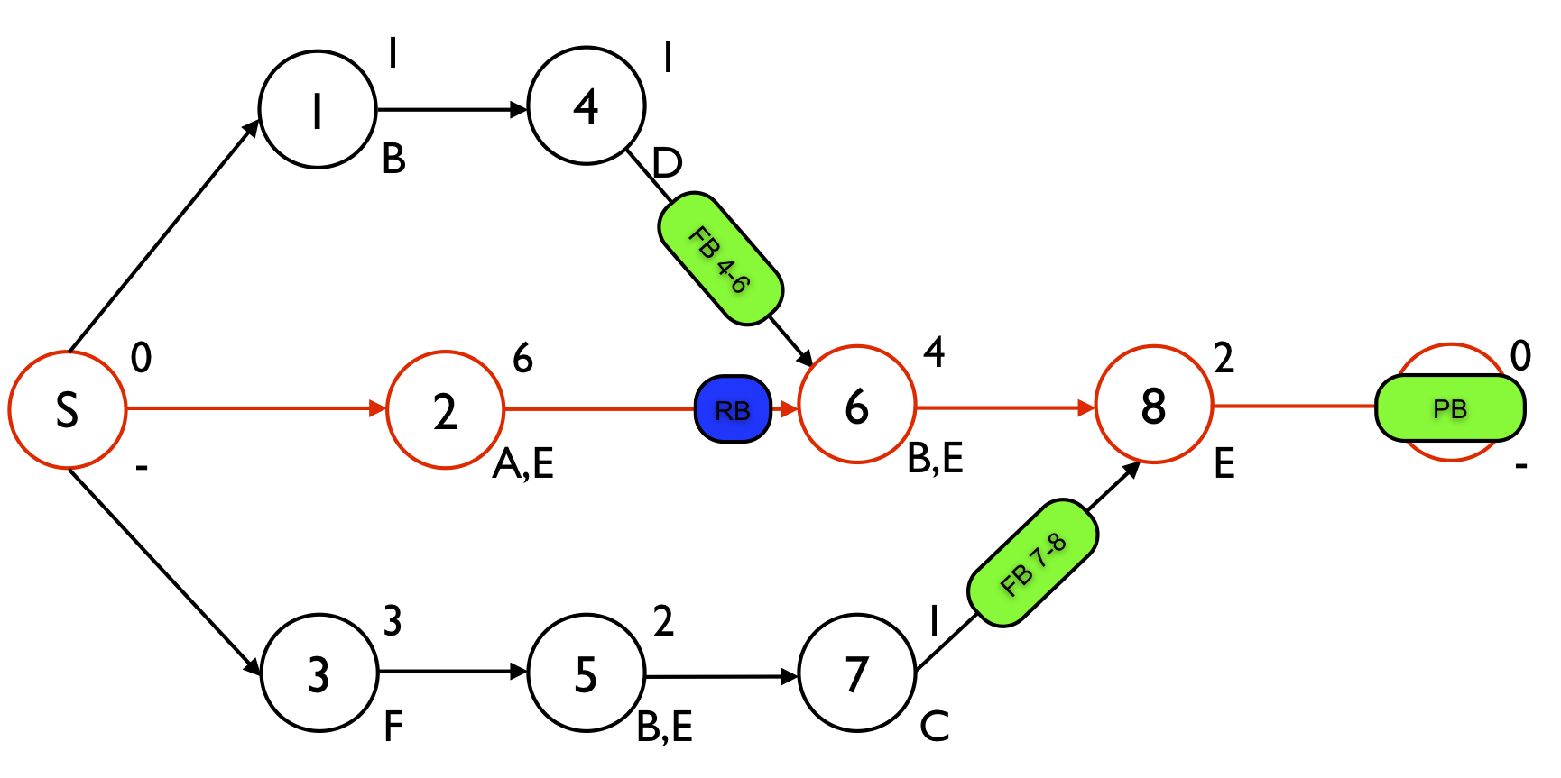
Figure 1 displays a project network with 8 activities. The numbers above each node are used to refer to the aggressive activity durations while the label below the node refers to a renewable resource that is required to perform the activity. The renewable resources A, B, C, D and F have an availability of one, while the renewable resource E availability is restricted to two units. The schedule contains three time buffers and one resource buffer. One project buffer is added to protect the critical chain S - 2 - 6 - 8 - E and two feeding buffers FB4-6 and FB7-8 are added to protect the feeding chains 1 - 4 and 3 - 5 - 7, respectively. The resource buffer RB is added to assure that resource B will be available on time to start with activity 6. More information on the determination of these buffers can be found at “Critical Chain/Buffer Management: Adding buffers to a project schedule”.
Figure 1. The project network with 2 feeding buffers, one resource and one project buffer
The adaptive procedure with resource tightness
The rationale behind buffer sizing methods based on resource information is that resources that are scarce often have a huge impact on the duration of activities and hence on potential delays. To that purpose, the so-called adaptive procedure with resource tightness (APRT) has been proposed that takes the scarceness or tightness of resources into account. Buffers are sized according to these resource tightness values to assure that a higher degree of resource tightness leads to a bigger buffer size to increase their power to absorb potential delays.
The buffer is sized as the standard deviation of the path leading to the buffer scaled by a factor which is calculated by taking the resource tightness into account, as follows:
Buffer size = K x σpath
with
K: The scaling factor based on the resource tightness.
σpath: The standard deviation of the longest path feeding the buffer.
buffer size
=
standard deviation of the path leading to the buffer scaled by a factor
which is calculated by taking the resource tightness into account.
In the following sections, the calculations of the path standard deviations, the resource tightness and the scale parameter K are illustrated on the example network of figure 1.
Standard deviation
The standard deviation of the longest path can be calculated in various ways. In this article, it is assumed that the standard deviations of the activities are equal to 50% of the difference between the safe and aggressive durations (see table 1). The standard deviation σpath of a path is then equal to the square root of the sum of the variances of the activities on that path, as follows:
- Critical chain 2 - 6 - 8: sqrt(1.52 + 12 + 0.52) = 1.87
- Feeding chain 1 - 4: sqrt(0.52 + 0.52) = 0.71
- Feeding chain 3 - 5 - 7: sqrt(12 + 0.52 + 0.52) = 1.22
More detailed calculations are given in “Critical Chain/Buffer Management: Sizing project and feeding buffers”.
Table 1. Aggressive and safe activity durations
| Activity | 1 | 2 | 3 | 4 | 5 | 6 | 7 | 8 |
| Safe duration | 2 | 9 | 5 | 2 | 3 | 6 | 2 | 3 |
| Aggressive duration | 1 | 6 | 3 | 1 | 2 | 4 | 1 | 2 |
Resource tightness
The resource tightness is a measure of the degree of resource use along the time horizon of all activities on the chain merging into the buffer. More precisely, it compares the total resource work content used by these activities with the total resource work content available during this time horizon for all resources.
- Total work content used by all activities on the chain: The work content is equal to the activity duration multiplied by the resource demand. As an example, the work content for activity 3 is equal to 3 * 1 = 3 for resource F.
- Total work content available along the length of the chain: The work content available is equal to the duration of the longest path in the chain multiplied by the resource availability of the resource. For example, this is equal to 12 * 2 for resource E of the critical chain.
For more information on the difference and use of the resource demand, resource availability and work content, see e.g. “Linking resources to activities: Resource availability and resource demand” and “The cost of a project activity: Calculating the activity and/or resource costs”.
The resource tightness is then calculated as the division of the two work contents, which leads to a value between 0 and 1, as follows:
- Resource tightness = total work content used / total work content available
Table 2 shows the resource tightness values for the different resources that are used for sizing the project buffer and the two feeding buffers.
These calculations are illustrated for resources A and E on the critical chain that has a length equal to 12 time units (e.g. days).
Resource A is only used by activity 2, and its total work content used is therefore equal to the duration of activity 2 multiplied by the resource demand, i.e. 6 * 1 = 6 (man days). The availability of resource A is equal to 1 and hence its total work content available is equal to 12 * 1 = 12. Consequently, the periodic resource tightness for resource A along the critical chain is equal to 6 / 12 = 0.5.
The resource demand for resource E is equal to one for all activities (2, 6 and 8) on the critical chain and the total work content used is then equal to (6*1 + 4*1 + 2*1) = 12. Its availability is equal to 2 and hence its total work content available is equal to 12 * 2 = 24. Consequently, the periodic resource tightness for resource E along the critical chain is equal to 12 / 24 = 0.5.
Table 2. Average resource use necessary to calculate the resource tightness
| Resource | PB | FB4-6 | FB7-8 |
| A | 6/12 | - | - |
| B | 4/12 | 1/2 | 2/6 |
| C | - | - | 1/6 |
| D | - | 1/2 | - |
| E | 12/24 | - | 2/12 |
| F | - | - | 3/6 |
| maximum | 6/12 = 0.5 | 1/2 = 0.5 | 3/6 = 0.5 |
The resource tightness is then set as the maximum of all resource tightness values of all resources used by the activities in the chain (as displayed in the last row in table 2)
Scale parameter K
The scaling factor K is equal to:
K = 1 + maximum resource tightness
The buffer sizes based on the adaptive procedure with resource tightness are then equal to:
- Project buffer: 1.5 * 1.87 = 2.81
- FB4-6: 1.5 * 0.71 = 1.07
- FB7-8: 1.5 * 1.22 = 1.83
The rationale behind this buffer sizing method that a higher average resource use and consequently a higher resource tightness is more risky and could possibly be the cause of delays makes sense. When the total resource use is close to the total resource availability, it is indeed more likely that delays will occur more often and therefore larger buffers should be added that are able to absorb these delays. An overview of other buffer sizing methods is available at “Critical Chain/Buffer Management: Sizing project and feeding buffers”.
© OR-AS. PM Knowledge Center is made by OR-AS bvba | Contact us at info@or-as.be | Visit us at www.or-as.be | Follow us at @ORASTalks
