
The Program Evaluation and Review Technique (PERT): Incorporating activity time variability in a project schedule
The Program Evaluation and Review Technique (PERT) is a project scheduling technique to analyze and represent the tasks involved in completing a given project. It incorporates activity duration variability and relies on similar concepts as the critical path method (CPM, see “The Critical Path Method (CPM): Incorporating activity time/cost trade-offs in a project schedule”).
Table 1: An example project for PERT calculations
| Task | Predecessors | a | m | b |
| A | none | 2 | 5 | 8 |
| B | A | 1 | 2 | 9 |
| C | A | 0.25 | 0.5 | 3.75 |
| D | B | 1 | 1 | 7 |
| E | B and C | 1 | 2 | 9 |
| F | D and E | 1 | 3 | 11 |
In this article, the technique will be explained by means of the example project data of table 1. More precisely, the following elements, necessary to analyze a PERT project network, will be discussed:
- The calculation of the activity duration estimates based on three input measures
- The calculation of the activity average and variance
- The calculation of the average critical path
- The use of the central limit theorem
- The presence of the normal distribution
Activity duration estimates
Activity durations are based on estimates made by human beings and are therefore error-prone. In PERT, the technique requires three duration estimates for each individual activity, as follows:
- Optimistic time estimate (a): This is the shortest possible time in which the activity can be completed, and assumes that everything has to go perfect
- Realistic time estimate (m): This is the most likely time in which the activity can be completed under normal circumstances
- Pessimistic time estimate (b): This is the longest possible time the activity might require, and assumes a worst-case scenario
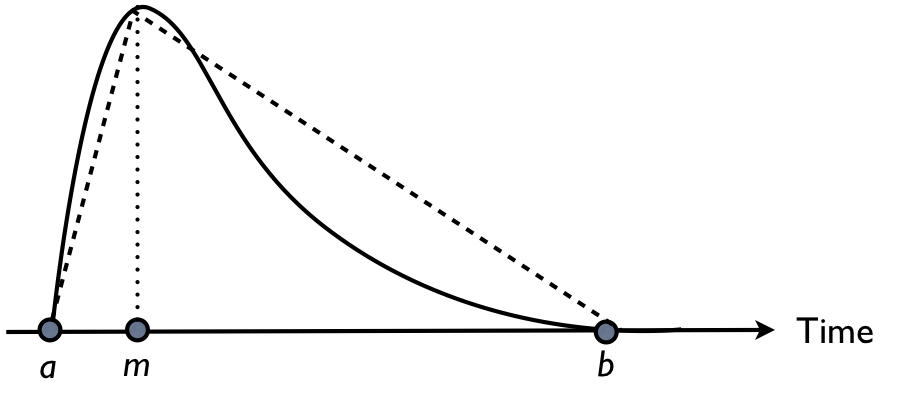
Figure 1: A PERT (solid line) and triangular (dotted line) distribution
Activity average and variance
Based on the three estimates, a weighted average and variance is calculated for each activity duration as a measure of the average duration and the corresponding variability, respectively. The weighted average is equal to (a + 4m + b) / 6 to express that the likeliness that the real activity duration lies close to the realistic estimate (m) is larger than the likeliness that it lies closer to the two extreme values a or b.
The standard deviation is equal to (b - a) / 6 and is based on the principles of a three-sigma interval that states that 99.73% (i.e. almost all) of the observations lie in that interval when the variable is normally distributed. Although it is assumed that the activity duration is beta distributed, the general principle is that the standard deviation assumes that almost all observations (i.e. real durations) will lie between the extreme values a and b.
The average durations and their standard deviations are given in the second line above each node of figure 2.
The average critical path
The expected duration D of a critical path is equal to the sum of the expected durations of the critical activities, i.e. E(D) = 5 + 3 + 3 + 4 = 15
The expected variance V of a critical path is equal to the sum of the variances of the critical activities, i.e. E(V) = 12 + (8/6)2 + (8/6)2 + (10/6)2 = 7.33. Note that only the activities on the (average) critical path are taken into account for the calculation of the variance.

Figure 2: The project network and the (average) critical path
The central limit theorem
The main idea of the central limit theorem (CLT) is that the average of a sample of observations drawn from a population with any distribution shape is approximately distributed as a normal distribution if certain conditions are met. More precisely, the central limit theorem states that given a distribution with a mean μ and variance σ², the sampling distribution of the mean approaches a normal distribution with a mean (μ) and a variance σ²/n as n, the sample size, increases. The amazing and counter-intuitive thing about the central limit theorem is that no matter what the shape of the original distribution is, the sampling distribution of the mean approaches a normal distribution.
In PERT, the project network of figure 2 represents the population, while the sample that is drawn from that population is equal to the average critical path (highlighted in red).
Consequently, the project duration follows a normal distribution with the following parameters:
- Average = E(D) = expected project duration (based on critical path)
- Variance = E(V) = expected variance (of the critical path)
The normal distribution
Using the characteristics of the normal distribution (N(15,7.33)) of the total project duration, basic statistical calculations can be applied to give answers to questions such as:
- What is the probability that the project will be finished before ...?
- What is the expected project deadline?
- What is a reasonable project duration such that it can be met with a probability of ... %?
As an example, the P(project duration ≤ critical path length E(D)) = 50% (symmetrical normal distribution) which clearly shows that the deterministic critical path underestimates the likely project duration.
Another example shows that the P(project duration ≤ 17) = P(z ≤ (17 - 15) / 2.71)) = P(z ≤ 0.74) = 77%
with E(D) = 15 and E(V) = 7.33 using the transformations from the normal distribution N(15,7.33) to a standardized normal distribution N(0,1). This value can be found using standardized normal tables or by the “=NORMDIST(17,15,SQRT(7.33),1)” function in Excel.
© OR-AS. PM Knowledge Center is made by OR-AS bvba | Contact us at info@or-as.be | Visit us at www.or-as.be | Follow us at @ORASTalks

i love pmknowledgecenter.com